Weekly Paper Notes — the Seminal Paper of the Week for the 2026-11-14 digest. Area: Databases.
Authors: P. Griffiths Selinger, M. M. Astrahan, D. D. Chamberlin, R. A. Lorie, T. G. Price (IBM Research, San Jose) Published: Proceedings of the 1979 ACM SIGMOD International Conference on Management of Data, Boston, pp. 23–34. DOI: 10.1145/582095.582099
Why the paper still matters
Codd’s relational model (our seminal pick in August) let users say what data they wanted and leave how to the system. That only works if the system picks a good “how” on its own. In the mid-1970s many people doubted it could, and a declarative language that ran ten times slower than hand-written navigational code would not have been adopted.
This paper is the answer IBM’s System R team gave. It is twelve pages long, and it describes an optimizer that estimates the cost of each candidate plan from statistics in the catalog, searches join orders with dynamic programming, and keeps extra plans when their output order can save a sort later. Every part of that sentence still describes the planner in Postgres, the cost-based optimizer in Spark, and the planners of most commercial databases.
The companion lakehouse paper in this week’s digest, Raven, is partly a fight over where per-file min/max statistics should live. Those statistics exist so that an optimizer of the kind described here can prune and cost scans.
The setup
System R had two layers. The Relational Data System (RDS) parsed and optimized SQL. The Research Storage System (RSS) stored tuples in pages within segments and maintained B-tree indexes. The RDS reached the RSS through a tuple-at-a-time interface, the RSI. A query block went through four phases: parsing, optimization, code generation, and execution. Optimization happened once at compile time and the resulting plan was stored for reuse.
The optimizer had two kinds of access path to choose from for each relation:
- A segment scan, which reads every page of the segment holding the relation.
- An index scan, which walks a B-tree in key order, either over the whole index or bounded by start and stop keys.
Predicates the RSS could evaluate itself, without returning tuples to the RDS, were called search arguments, or SARGs. The word “sargable” that DBAs still use for an index-friendly predicate comes from this paper.
The cost model
Every plan’s cost is a weighted sum of I/O and CPU:
COST = PAGE FETCHES + W × (RSI CALLS)
RSI calls stand in for CPU work, since each one returns a tuple to the RDS. W is a tunable weight. To estimate both terms, the optimizer reads a small set of statistics from the catalog:
- NCARD(T), the number of tuples in relation T, and TCARD(T), the number of pages that hold them.
- P(T), the fraction of the segment’s pages that contain T’s tuples.
- ICARD(I), the number of distinct keys in index I, and NINDX(I), the number of pages in the index.
Statistics were refreshed by an explicit UPDATE STATISTICS command, not on every write, so the optimizer always planned from somewhat stale numbers. That trade-off is still how most systems work (ANALYZE in Postgres, ANALYZE TABLE ... COMPUTE STATISTICS in Spark).
The paper then gives each predicate a selectivity factor F, the expected fraction of tuples that satisfy it:
| Predicate | F |
|---|---|
column = value |
1 / ICARD(index), or 1/10 with no index |
column1 = column2 |
1 / max(ICARD₁, ICARD₂), or 1/10 with no index |
column > value |
(high key − value) / (high key − low key), or 1/3 |
column BETWEEN v1 AND v2 |
(v2 − v1) / (high key − low key), or 1/4 |
p AND q |
F(p) × F(q) |
p OR q |
F(p) + F(q) − F(p) × F(q) |
NOT p |
1 − F(p) |
Two assumptions are built into the table. Values are uniformly distributed between the low and high key, and predicates are independent, so ANDed selectivities multiply. Both are often wrong on real data, and most of the next 45 years of optimizer research went into fixing them. The default constants also lasted a long time. Postgres still falls back to a selectivity of one-third for an inequality it has no statistics for.
The expected output size of a query block is then the product of the cardinalities of the relations in its FROM list times the selectivities of its predicates.
The algorithm walk-through
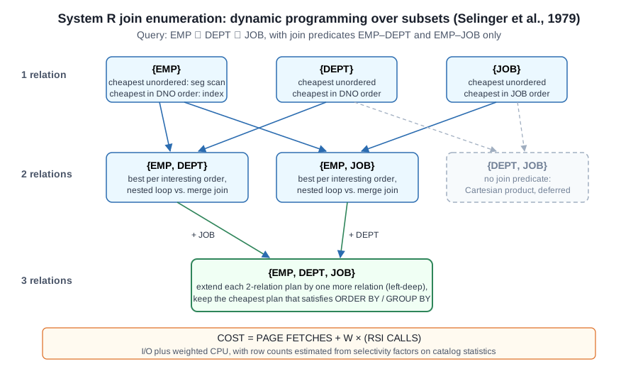
 Figure: Join enumeration for a three-relation query. Each box keeps the cheapest plan for that set of relations for each interesting order, plus the cheapest unordered plan. Original diagram for this post.
For a single relation, the optimizer costs each access path and keeps the cheapest one. It also keeps the cheapest path for each interesting order. An order is interesting if the query’s GROUP BY or ORDER BY needs it, or if a later join could use it. An index scan on EMP.DNO may cost more than a segment scan, but if the plan will merge-join on DNO or sort by DNO afterward, reading in DNO order can make the whole plan cheaper. This is why the optimizer can’t just keep the single cheapest plan for each subset.
For joins, the paper considers two methods. A nested-loop join scans the inner relation once for each outer tuple, which is cheap when the inner side has an index on the join column. A merge join (the paper calls it “merging scans”) needs both inputs sorted on the join column and walks them together.
The search is the part that later systems copied most directly. Plans are built bottom-up by number of relations:
- Find the best way to access each single relation, per interesting order.
- For each pair of relations, find the best way to join them, using the stored single-relation plans as building blocks, again per interesting order.
- For each set of k relations, extend the stored (k−1)-relation plans by joining one more relation, and keep the best result per interesting order.
Because the optimizer remembers the best plan for each subset and order, it never re-derives a sub-plan, and the search costs on the order of 2ⁿ subsets instead of n! join orders. Two heuristics shrink it further. Joins are always left-deep, meaning the inner input is a single base relation, never an intermediate result. And a relation is only joined to the current set if a join predicate connects them, so Cartesian products are deferred until no other option is left. In the diagram, {DEPT, JOB} is never built, because no predicate links DEPT and JOB.
The paper also covers nested queries. An uncorrelated subquery is evaluated once and its result reused. A correlated subquery, which references a column of the outer query, has to be re-evaluated for each candidate outer tuple, though System R avoided recomputing it when consecutive outer tuples carried the same referenced value.
What the paper doesn’t claim
The authors don’t say the cost estimates are accurate in absolute terms. Their claim is that the ordering is usually right: on their test queries, the plan the optimizer ranked cheapest was usually also the fastest when executed. For a component whose job is to choose a plan, getting the ranking right matters more than getting the numbers right.
Left-deep trees and deferred Cartesian products are presented as heuristics that shrink the search, not as theorems. Both are wrong for some queries. Star-schema joins, for example, sometimes do best by crossing small dimension tables first, and bushy plans can win on parallel hardware.
Why this design has outlasted everything around it
System R’s storage engine, its tuple-at-a-time interface and its locking design have all been replaced. The optimizer’s structure is still in use:
- Postgres enumerates join orders with the same bottom-up dynamic programming, switching to a genetic search (GEQO) once a query has more than
geqo_thresholdrelations (12 by default). It also keeps paths with useful sort orders (“pathkeys”) alongside the cheapest unsorted path, which is the interesting-orders idea. - Spark SQL’s cost-based optimizer reorders joins with a dynamic-programming algorithm of the same kind, guarded by a similar size threshold, and uses table and column statistics collected by
ANALYZE TABLE. - Volcano and Cascades (Graefe, 1993 and 1995), which underlie SQL Server and several newer engines, changed how the plan space is generated (top-down, rule-driven, memoized), but they kept costing each plan from statistics and choosing the cheapest.
The weak point has stayed the same too. Leis et al.’s How Good Are Query Optimizers, Really? (VLDB 2015) found that bad plans come mostly from cardinality estimation errors, caused by the uniformity and independence assumptions in the selectivity table above, and much less from the cost model or the search. Histograms, sampling, multi-column statistics, adaptive execution and learned estimators are all attempts to fix that one table of selectivity factors.
Read alongside
- Astrahan et al., System R: Relational Approach to Database Management (ACM TODS, 1976): the system this optimizer was built for.
- Chamberlin and Boyce, SEQUEL: A Structured English Query Language (1974): the language that became SQL.
- Graefe, The Cascades Framework for Query Optimization (IEEE Data Eng. Bull., 1995): the main structural alternative to bottom-up dynamic programming.
- Chaudhuri, An Overview of Query Optimization in Relational Systems (PODS, 1998): a survey of what was built on top of this paper over twenty years.
- Leis et al., How Good Are Query Optimizers, Really? (VLDB, 2015): a measurement of where Selinger-style optimizers still go wrong.
- Marcus et al., Bao: Making Learned Query Optimization Practical (SIGMOD, 2021): learning to steer a classic optimizer instead of replacing it.
Links
📄 ACM Digital Library (DOI: 10.1145/582095.582099)
Part of the Weekly CS Paper Digest series. Written from the published paper; the diagram is original to this post.