Weekly Paper Notes — the Seminal Paper of the Week for the 2026-11-07 digest. Area: AI / ML.
Authors: David E. Rumelhart (UC San Diego), Geoffrey E. Hinton (Carnegie Mellon University), Ronald J. Williams (UC San Diego) Published: Nature 323, 533–536, 9 October 1986. DOI: 10.1038/323533a0
Why the paper still matters
Every model in this week’s digest was trained by the procedure this letter describes: run the network forward, measure the error, push its derivative backward layer by layer, and nudge every weight downhill. Every gradient that JAX’s grad or PyTorch’s loss.backward() computes is reverse-mode differentiation, and this paper is the one that showed neural networks what it could do.
Earlier work had a specific gap. By 1986 there were good learning rules for networks where inputs connect straight to outputs: the perceptron convergence procedure, the delta rule. Minsky and Papert’s Perceptrons (1969) had shown how limited those networks are. A single layer can’t tell whether a bit pattern is a palindrome, or compute XOR. Hidden units fix the expressiveness, but nobody had a general way to train them. The task specifies what the outputs should be. It says nothing about what a hidden unit should be doing.
The paper’s claim, in its own words, is that “a general purpose and relatively simple procedure is powerful enough to construct appropriate internal representations.” The title says learning representations, not learning weights, and that choice of emphasis is the main thing the paper contributed.
The procedure
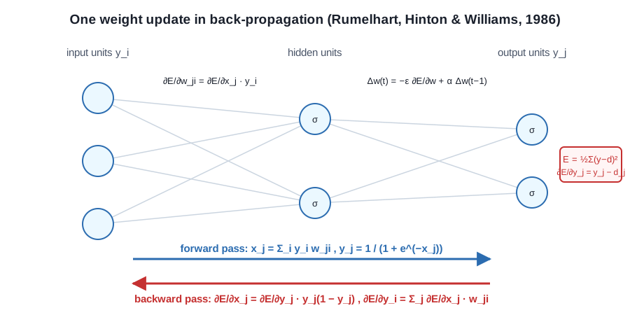
The setup takes a paragraph. Each unit computes a weighted sum of its inputs, x_j = Σ_i y_i w_ji, and passes it through a logistic sigmoid, y_j = 1 / (1 + e^(−x_j)). Biases are weights from an always-on unit. The error over a training set is squared distance from the targets, E = ½ Σ_c Σ_j (y_j,c − d_j,c)².
 The forward pass computes activations; the backward pass reuses them to get every weight’s gradient in one sweep. Original diagram for this post.
The backward pass is where the cost saving comes from. At an output unit, ∂E/∂y_j = y_j − d_j. Multiply by the sigmoid’s derivative, which is just y_j(1 − y_j) and so needs nothing beyond what the forward pass already computed, and you have ∂E/∂x_j. From there:
∂E/∂w_ji = ∂E/∂x_j · y_i                 (gradient for the weight from i to j)
∂E/∂y_i  = Σ_j ∂E/∂x_j · w_ji            (error signal handed to the layer below)
Apply the second line at each layer and the error signal moves down the network, producing every weight’s gradient along the way. The total cost is about one extra forward pass, however many weights there are. Perturbing each weight separately to estimate its effect would cost one forward pass per weight.
The update rule is gradient descent with what we now call momentum: Δw(t) = −ε ∂E/∂w(t) + α Δw(t−1). The authors describe it as using the gradient to change the velocity of the point in weight space rather than its position. They accumulate gradients over the whole training set before each step (full-batch), and they start from small random weights “to break symmetry”, because if every hidden unit starts identical, every hidden unit gets the same gradient and they stay identical forever.
Two demonstrations
The paper earns its title with two small experiments.
Mirror symmetry. Six binary inputs, and the task is to say whether the pattern is a palindrome. No single input carries any evidence on its own, so no direct input-to-output rule can work. A network with only two hidden units learned it in 1,425 sweeps through the 64 possible inputs. The solution it found is neat. Each hidden unit gives mirror-image inputs weights of equal size and opposite sign, so a symmetric pattern sums to zero. The weights on each side are in the ratio 1:2:4, so every half-pattern produces a unique sum and only its exact mirror can cancel it. The two hidden units are sign-flipped copies of each other, so any asymmetric pattern turns one of them on, and that suppresses the output. Nobody designed this. Gradient descent found a binary-encoding trick.
Family trees. Two isomorphic family trees, one English and one Italian, each with twelve people, are encoded as triples like (Colin, has-aunt, ?). People and relationships are presented as one-hot inputs: 24 units for people, 12 for relationships. Each feeds its own 6-unit layer, then a 12-unit central layer, then 6 units, then 24 outputs. Trained on 100 of the 104 triples, the network answered the 4 held-out ones correctly.
Its six-unit encoding of people is the important part. One unit learned English versus Italian. Another learned generation. Another learned which branch of the family a person belongs to. None of those features appear in the input, which gives every person an unrelated one-hot code. Because English and Italian people with the same role got almost the same representation, what the network learned about one tree carried over to the other. This is a learned embedding, in 1986, and it generalised for the reason embeddings still do.
What the paper doesn’t claim
The paper is careful about its limits, which helps explain why it holds up.
It doesn’t claim to have invented the method. It says variants were “discovered independently by David Parker… and by Yann Le Cun.” The full history goes back further. Seppo Linnainmaa described reverse-mode automatic differentiation in his 1970 master’s thesis. Paul Werbos proposed applying it to neural networks in his 1974 PhD thesis and worked it out more fully in 1982. The 1986 paper’s contribution was showing that the procedure produces useful internal representations, and saying so in Nature, where the whole field would read it.
It names the obvious drawback, local minima, and answers from experience: networks “very rarely” get stuck in poor ones, and adding a few connections opens paths around the barriers. Overparameterisation smoothing the loss landscape is now a research area of its own.
It treats recurrent networks too. A network run for several time steps is equivalent to a deep layered network with tied weights, so the same procedure trains it, as long as you store each step’s activations and average the gradients over the tied copies. That’s backpropagation through time, in one figure caption.
It also says the procedure “is not a plausible model of learning in brains”. Hinton spent much of the next four decades looking for one that is.
What happened next
The companion chapter in the Parallel Distributed Processing volumes (Rumelhart, Hinton and Williams, “Learning internal representations by error propagation”) gave the full derivation and many more experiments, and the two together started the connectionist boom of the late 1980s. NETtalk learned to read English text aloud in 1987. LeCun’s 1989 network read handwritten ZIP codes for the US Postal Service, and adding convolution and weight sharing to backprop produced the CNN.
Then the method ran into its limits. Hochreiter’s 1991 thesis showed that gradients in deep and recurrent networks vanish or explode as they pass through many sigmoid layers. Compute was scarce and labelled data scarcer, and SVMs and graphical models took over much of machine learning for over a decade. The fixes came one at a time: LSTMs (1997), layer-wise pretraining (2006), ReLUs, GPUs, ImageNet, and AlexNet in 2012. None of them replaced backprop. They made it work at larger depth and scale.
Today the algorithm is everywhere, in nearly the same form. Squared error became cross-entropy, sigmoids became GELUs, full-batch descent became Adam on minibatches, and hand-derived backward passes became automatic differentiation, but the forward pass, backward pass and gradient step are what this paper describes. Hinton shared the 2018 Turing Award with LeCun and Bengio and the 2024 Nobel Prize in Physics with John Hopfield. Rumelhart, who died in 2011, didn’t live to see the method take over the field.
The paper is still worth reading. It’s four pages long, the mathematics is the chain rule, and the two experiments show the thing people still argue about in LLM interpretability: features that no one specified appearing in hidden units because they reduce error.
Read alongside
- Rumelhart, Hinton, Williams, “Learning Internal Representations by Error Propagation”, in Parallel Distributed Processing, Vol. 1 (MIT Press, 1986): the long version with full derivations.
- Werbos, Beyond Regression: New Tools for Prediction and Analysis in the Behavioral Sciences (PhD thesis, Harvard, 1974): the earliest proposal to train neural networks this way.
- Minsky, Papert, Perceptrons (MIT Press, 1969): the limits that hidden units and backprop were answering.
- LeCun et al., Backpropagation Applied to Handwritten Zip Code Recognition (Neural Computation, 1989): backprop plus convolution.
- Baydin et al., Automatic Differentiation in Machine Learning: a Survey (JMLR, 2018): how reverse mode became the general tool behind modern frameworks.
Part of the Weekly CS Paper Digest series. Written from the published paper and its well-documented history; the diagram is original to this post.