Weekly Paper Notes — one of the top picks from the 2026-08-29 CS paper digest. Area: AI / Machine Learning.
Authors: Lukas Kuhn, Lucas Maes, Giuseppe Serra, Quentin Le Lidec, Yann LeCun, Randall Balestriero, Florian Buettner (German Cancer Research Center / DKTK / Goethe University Frankfurt, Mila, Université de Montréal, Brown University, Courant Institute NYU, AMI Labs) arXiv: 2608.27395 · PDF · Project page
TL;DR
Self-supervised video encoders have been expensive twice over: video carries an order of magnitude more tokens than an image, and the dominant methods add machinery on top of that cost purely to keep representations from collapsing. V-JEPA maintains an exponential-moving-average target encoder, a stop-gradient, and a predictor network over masked queries; masked autoencoders instead sidestep collapse by reconstructing pixels through a decoder. Neither the target-encoder forward pass nor the decoder contributes to the representation you actually keep.
LeVJEPA removes both by porting LeJEPA’s SIGReg objective — which excludes collapse with a provable guarantee rather than an architectural trick — to video. What remains trainable is an encoder and a small projector. The loss is a mean squared error pulling local-view embeddings toward a global-view embedding, plus SIGReg, with a single hyperparameter fixed to its published default (λ = 0.02) in every experiment reported. Two consequences follow. First, since step cost is now governed only by the number of tokens the encoder sees, tokens can be dropped aggressively: at 95% uniform random dropping, ImageNet-1K attentive-probe accuracy rises to 47.6% from 33.9% at zero dropping. Second, with no branch asymmetry to maintain, attention topology is unconstrained, so the encoder trains with block-causal attention at no accuracy cost (51.2% vs. 50.7% bidirectional). At matched epochs on identical data, LeVJEPA matches or beats V-JEPA 2 across ViT-S/B/L at 5.6–20.8x less total pretraining compute; at matched FLOPs it leads the strongest video baseline by 7.6 points on ImageNet.
What problem is the paper actually attacking?
The lineage matters here, because the paper is arguing that a decade of accumulated design conventions were downstream of a single problem that now has a cleaner solution.
Joint-embedding methods map augmented views of an input to nearby representations, and the constant function is always an available cheat. BYOL showed you could exclude it without negative pairs by breaking symmetry: an online branch and an EMA target branch, a stop-gradient, a predictor head. DINO adopted the same teacher–student arrangement with centering and sharpening, and contributed multi-crop — several aggressively cropped local views matched against a small number of global views. V-JEPA carried this to video and added masked-token prediction in latent space. The mechanisms work empirically, but they introduce extra networks and schedules whose effect on learning dynamics is hard to characterize, and there is no analytical guarantee that collapse is excluded.
Masked pixel reconstruction took the other road. Because imputing held-out pixels admits no trivial solution, no collapse prevention is needed at all. But VideoMAE observed that natural video’s temporal redundancy makes naive masking too easy — content hidden at one instant can simply be copied from an adjacent frame — and introduced tube masking, occluding the same spatial region across every frame, which then permits 90–95% masking ratios. The paper’s sharpest observation is about this artifact: the tube pattern is a property of the imputation task, not of video. It was inherited by methods that no longer impute anything, and once you stop imputing, it becomes actively harmful.
The motivating observation, then: if collapse can be excluded by an explicit distributional constraint with a proof attached, every component that exists only to stabilize learning can be deleted, and the masking scheme can be redesigned around what video actually needs.
The mechanism: one encoder, invariance plus SIGReg
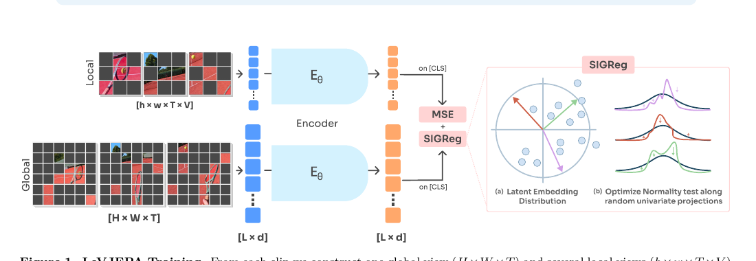
![LeVJEPA training. One global view and several local views share a temporal window; 95% of patch tokens are dropped uniformly at random; both views pass through the same shared block-causal encoder; the loss reads only the [cls] embedding, combining MSE toward the global embedding with SIGReg, which projects the batch onto random directions and penalizes deviation from a standard Gaussian. Source: Kuhn et al. — arXiv:2608.27395, Figure 1.](fig-lev-arch.png)
From a video, sample a 16-frame clip and build V+1 views: one global view at full resolution, and V local views produced by aggressive spatial cropping and photometric augmentation. All views share the identical temporal window and differ only spatially and photometrically. Every view goes through the same encoder Eθ; a learnable [cls] token gives the clip-level readout, which a small projector hϕ maps into a K-dimensional embedding space. The projector is not decoration — the encoder’s final layer applies layer normalization, which pins the [cls] representation to a sphere and would prevent SIGReg from being optimized in the encoder’s output space. It is discarded after pretraining.
The objective is
L = L_inv + λ · L_SIGReg
with the invariance term the plain mean squared error between the global embedding and each local one:
L_inv = (1/(V+1)) · Σ_v ‖z₀ − z_v‖²₂
Gradients flow through both arguments — z₀ comes from the same encoder in the same forward pass as the local embeddings, with no stop-gradient and no target network. Minimized alone, this obviously collapses.
SIGReg is what excludes that. It constrains the embedding distribution to an isotropic Gaussian, the distribution Balestriero and LeCun show minimizes worst-case downstream probing risk, and from which any collapsed solution — having zero variance along some direction — is maximally distant. The high-dimensional constraint is made tractable by the Cramér–Wold theorem: embeddings match N(0, IK) if and only if every one-dimensional projection matches N(0,1). So each step samples M directions uniformly on the sphere SK−1 and penalizes each projected batch’s deviation from a standard Gaussian using the Epps–Pulley statistic:
L_SIGReg = (1/M) · Σ_m ∫ |(1/n)Σ_i e^{it⟨z_i,a_m⟩} − e^{−t²/2}|² e^{−t²/2} dt
approximated by quadrature. The empirical characteristic function underlying this is bounded with bounded gradients, which makes the loss robust to outliers, free of whitening or centering, and cheap to evaluate distributed across the full global batch.
Two architectural choices follow from having no asymmetry to preserve. Tokenization is per frame — the convolutional patch embedding has spatial extent 16×16 and temporal extent τ = 1 by default, so no temporal aggregation is imposed at the input (3,136 tokens for a 224² global view, 576 for a 96² local view). Attention is block-causal: patch tokens attend bidirectionally within their own frame and causally to preceding frames, while the [cls] token attends to everything but is never attended to. A frame’s representation is therefore a function of current and past frames only. Factorized 3D rotary embeddings encode relative position, letting one encoder handle both view resolutions without interpolation. The [cls] token receives the objective exclusively and is never dropped; patch tokens get no direct supervision at all.
Why pretraining gets cheap
Because every operation now contributes to the objective, step cost reduces to a single quantity: how many tokens the encoder observes. That makes the observed token set a free parameter of the method rather than a component of a prediction task — and the paper pushes it hard.
Dropping ρ = 0.95 of patch tokens uniformly at random after patch embedding cuts feed-forward cost by up to (1−ρ)⁻¹. If dropping were merely an efficiency approximation you would expect accuracy to fall. It rises monotonically: 33.9% at ρ = 0, 39.6% at 0.3, 44.8% at 0.6, 47.6% at 0.95. Dropping is acting as a stochastic augmentation, forcing the clip-level embedding to be inferable from a sparse, randomly located sample of the clip. And ρ = 0.9 versus ρ = 0.95 are indistinguishable (47.4% vs. 47.6%), so halving the processed tokens again costs nothing — the most aggressive setting is also the most economical.
The comparison against tube dropping is where the inherited-convention argument pays off. Retaining identical spatial locations in every frame, mirroring the space-time masks of masked video modeling, drops ImageNet accuracy from 50.7% to 39.6%, with the same ordering on Something-Something-v2. The explanation is clean: under masked prediction, structured masks are necessary to keep imputation non-trivial, since randomly scattered masks let the model interpolate from spatial neighbors. Here nothing is imputed — the retained tokens are the encoder’s only observation of the clip — so a tube pattern permanently occludes most of the scene in every frame, while uniform random dropping yields a spatio-temporally distributed sample from which clip content stays identifiable.
The memory consequence is what makes the accessibility claim land. On a 16 GB RTX 5080, LeVJEPA trains at batch size 128 in under 8 GB, whereas a V-JEPA configuration with an identically sized encoder saturates the card at batch size 28. A ViT-Tiny trained for 12 hours on that single consumer GPU, on eight unlabeled Walking Tours egocentric videos (~620k frames, ~5M clips), lifts frozen ImageNet top-1 from 8.9% at initialization to 25.2%.
Results
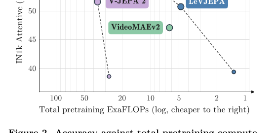
All baselines are retrained on the identical 20% K710 subsample with their official implementations and recommended hyperparameters, for the same 240 epochs at the same effective batch size of 3,072 — which removes the usual confound of comparing against numbers trained on different data for different schedules. Evaluation is frozen attentive probing following V-JEPA’s protocol exactly, with sequence length equalized across methods so nobody is probed on more tokens than anyone else.
Under the epoch-matched protocol, LeVJEPA tracks or exceeds V-JEPA 2 at every model size while using far less compute: 20.8x less at ViT-S, 5.6x at ViT-L. At ViT-B the two are within one accuracy point while LeVJEPA consumes 4.8 ExaFLOPs against 36.4. At ViT-L it stops being merely comparable and passes V-JEPA 2 by 1.9 points — and the LeVJEPA ViT-L costs less than half what the V-JEPA 2 ViT-S did. VideoMAEv2 sits between the two methods on both axes.
The FLOP-matched table is the stronger result and also the more nuanced one. Holding total compute equal grants LeVJEPA a much longer schedule (1,085 epochs, V = 10 local views). It takes ImageNet by 7.6 points (61.0 vs. VideoMAEv2’s 53.4 and V-JEPA 2’s 51.6) and K400 linear probing by a smaller margin (44.6 vs. 40.7 and 37.4) — but loses Something-Something-v2, at 40.4 against VideoMAEv2’s 43.6 and V-JEPA 2’s 42.5. The paper’s phrasing is “remains competitive,” which is fair, though it is worth naming that the one benchmark most dependent on fine-grained motion is the one where the method does not win.
That gap is consistent with the ablation’s own caveat. While ImageNet accuracy climbs monotonically with dropping ratio, SSv2 accuracy declines beyond ρ = 0.3. The authors report that longer training recovers it — higher dropping ratios eventually reach the accuracy of lower ones on SSv2 while keeping their lower per-iteration cost — and offer the plausible reading that sparse random observations make motion cues, which depend on cross-frame correspondence, less frequently recoverable within a single view. Dropping schemes that preserve motion information at high sparsity are left to future work, which is the right place to leave it and an honest way to flag it.
Three secondary results round out the picture. Temporal patch aggregation at the input, conventional since ViViT, turns out to be unnecessary: at matched token budgets, per-frame patching (τ = 1, ρ = 0.95) beats τ = 2, ρ = 0.90 on both IN1K (50.7 vs. 47.4) and SSv2 (30.4 vs. 28.8) — notably including the motion benchmark that aggregation is usually justified by. Block-causal attention matches bidirectional (51.2 vs. 50.7), so frame representations become computable from past observations alone, extending to incoming frames at constant incremental cost without re-encoding. And against a DINOv2 trained at equal total FLOPs on individual frames of the same videos, the image-pretrained encoder keeps a 3.1-point ImageNet advantage (53.8 vs. 50.7) while the video-pretrained one nearly doubles it on SSv2 (30.4 vs. 16.9).
A note on the patch-token PCA figure: the three leading principal components of LeVJEPA’s patch representations separate the animal from background furniture as cleanly as V-JEPA 2.1, which gets its dense structure from an explicitly added patch-level loss. V-JEPA 2, trained without that loss, shows no comparable organization. LeVJEPA’s structure emerges even though only the [cls] token is ever supervised.
Why this matters
The efficiency numbers will get quoted, but the interesting claim is about substrate. Video has always been the theoretically preferable source of visual representations — abundant, unlabeled, carrying motion, causality, and object permanence that static images cannot supply — and practically the expensive one. If the appearance-side cost of video pretraining shrinks to a few points at equal compute while the motion-side advantage stays decisive, the calculus flips, and the FLOP-matched DINOv2 comparison is the paper’s attempt to establish exactly that boundary condition.
The block-causal result may prove the more durable contribution. Bidirectional video encoders can only approximate streaming behavior by re-encoding a window or by fitting a separate temporal model after pretraining. An encoder whose frame representations depend only on past frames extends a video representation frame by frame at constant incremental cost — which is what autoregressive world models and streaming inference actually need. That this costs nothing in downstream accuracy is a genuinely useful negative result.
There is also a methodological argument running underneath. Each removed component — the EMA target, the stop-gradient, the predictor, the structured mask, temporal patch aggregation — was individually reasonable when introduced, and each was inherited by successors that no longer had the problem it solved. The tube-masking reversal is the cleanest demonstration: the same design that was necessary for masked prediction is harmful here, and only an ablation asking the question directly would have surfaced it. The obvious follow-up is whether the same audit, run against text or audio joint-embedding pipelines, turns up equally load-bearing fossils.
Read alongside
- Balestriero and LeCun, LeJEPA — the SIGReg objective and the isotropic-Gaussian argument that LeVJEPA transfers to video.
- Bardes et al., V-JEPA / V-JEPA 2 — the target-encoder-plus-predictor recipe being displaced, and the frozen attentive-probing protocol reused unchanged for evaluation.
- Tong et al., VideoMAE (NeurIPS 2022) and Wang et al., VideoMAEv2 (CVPR 2023) — where tube masking comes from, and why it was necessary there.
- Grill et al., BYOL (2020) and Caron et al., DINO (2021) — the origin of the asymmetry-based collapse prevention and of multi-crop.
- Oquab et al., DINOv2 (2023) — the image-pretraining baseline in the FLOP-matched comparison.
- Venkataramanan et al., Walking Tours — the uncurated egocentric footage used for the single-GPU experiment.
Links
📄 arXiv abstract · 📄 PDF · 💾 code and models
Part of the Weekly CS Paper Digest series. Summary written from a close read of the preprint; figures cropped from the arXiv PDF and reproduced here under fair use for educational commentary.