In early 2019 the Transformer was two years old. BERT and GPT existed, but most NLP courses still taught LSTMs as the default. Ashish Vaswani, first author of Attention Is All You Need, came to Stanford’s CS224N as its first guest lecturer that term and spent half an hour explaining why self-attention works, what it costs, and which inductive biases it brings. Anna Huang, lead author of the Music Transformer, gave the second half, on using relative attention to generate piano music. It’s the Classic of the Week because it’s one of the clearest explanations of the Transformer from the people who built it, given before scaling made the architecture look inevitable, so the reasoning is still visible.
Start from the structure of your data
Vaswani introduces himself as an empiricist and frames the lecture around a question he says he always asks first: what structure and symmetries are in the data, and is there a model whose inductive bias matches them? His argument is that self-attention has biases worth having, apart from being fast.
He’s specific about what was wrong with RNNs. Recurrence is sequential, so it limits parallelism, and he quotes Oliver Selfridge’s Pandemonium to the effect that more parallel computation just means you’ll add more data. Everything a recurrent network has read gets squeezed into one fixed-size vector, and it has no explicit way to represent hierarchy. Convolutional sequence models such as ByteNet and WaveNet parallelize trivially within a layer, but connecting distant positions still takes a number of layers that grows with distance, linearly or logarithmically with dilation. Attention was already the key mechanism in neural machine translation, as content-based retrieval from encoder to decoder. The question his group asked was “why not just use attention for representations?”
The Transformer, piece by piece

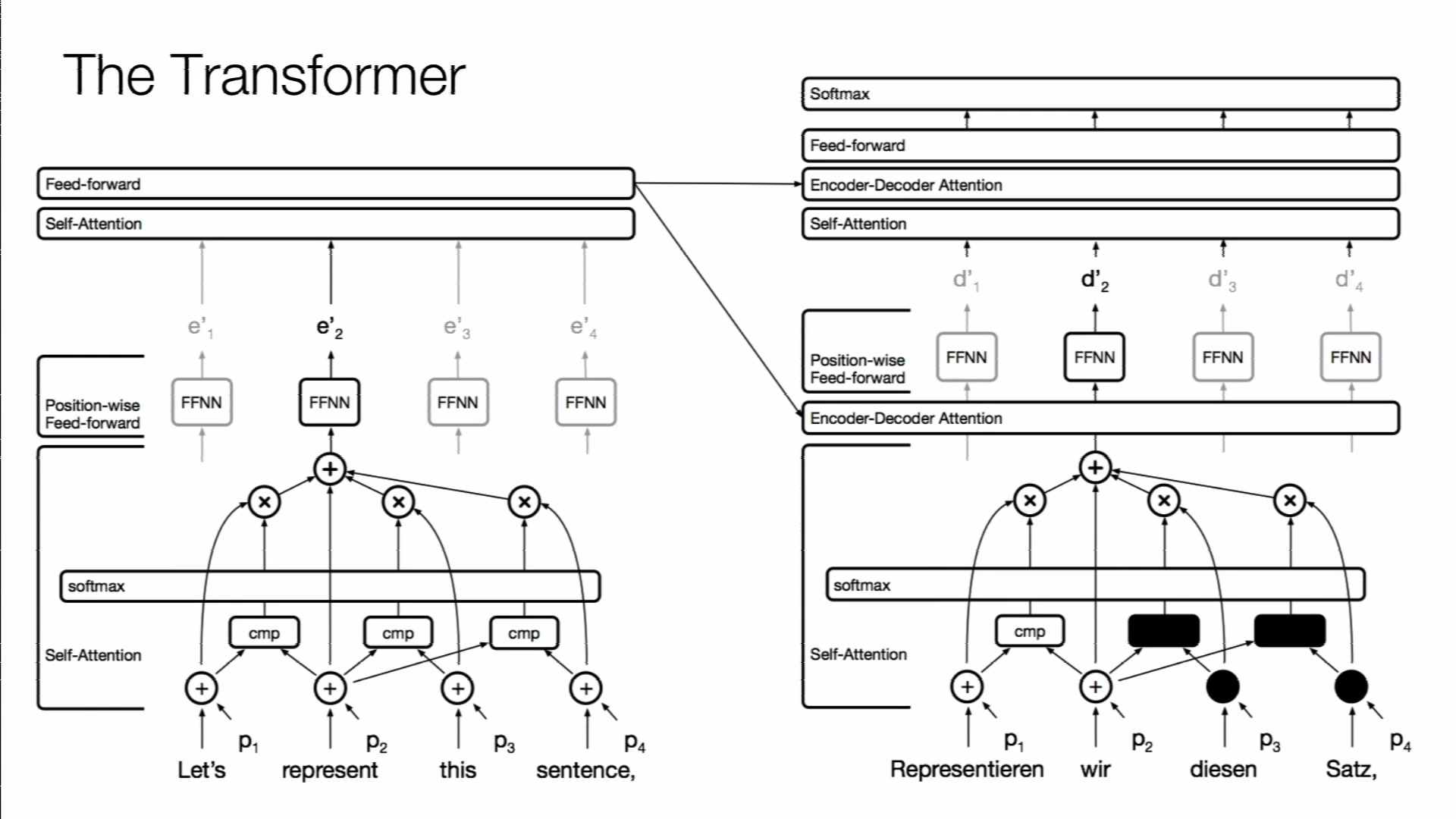
Attention doesn’t care about order, so positions are added at the input, either as the sinusoids (which he credits to Noam Shazeer) or as learned embeddings. “Both of them work equally well.” An encoder layer is self-attention followed by a feed-forward layer, with residual connections around each. The decoder is a language model built from self-attention, made causal by masking future positions, followed by attention to the final encoder layer and a feed-forward layer.
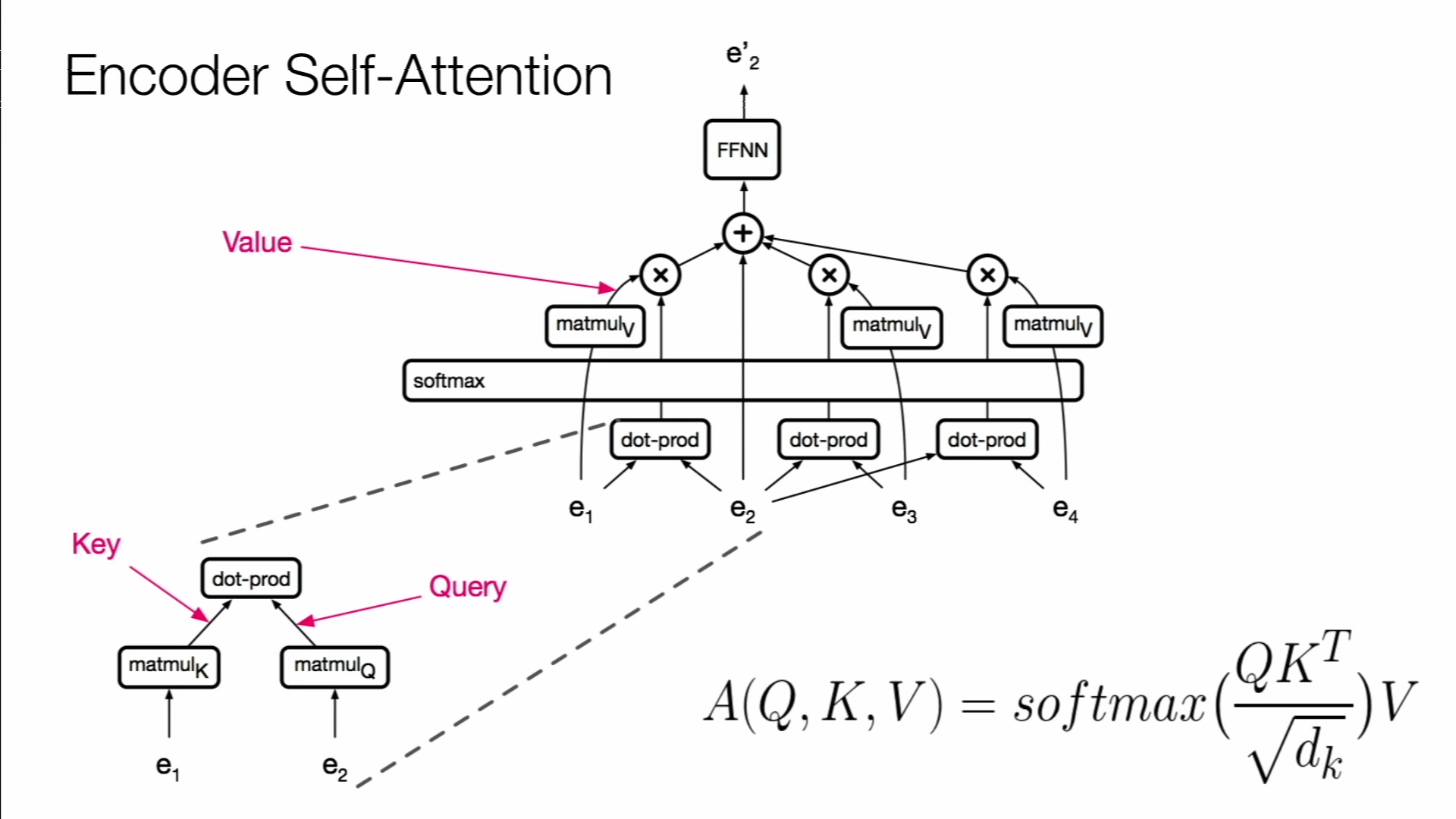
The mechanism was chosen “for simplicity and speed”. Project the position into a query and every other position into a key, take dot products, apply a softmax, and use the resulting convex combination to mix projected values. The whole thing is two matrix multiplications and a softmax for every position at once. The square-root scaling stops the dot products from growing too large. Causal masking is done by adding −10⁹ to the logits for future positions so they get zero probability.
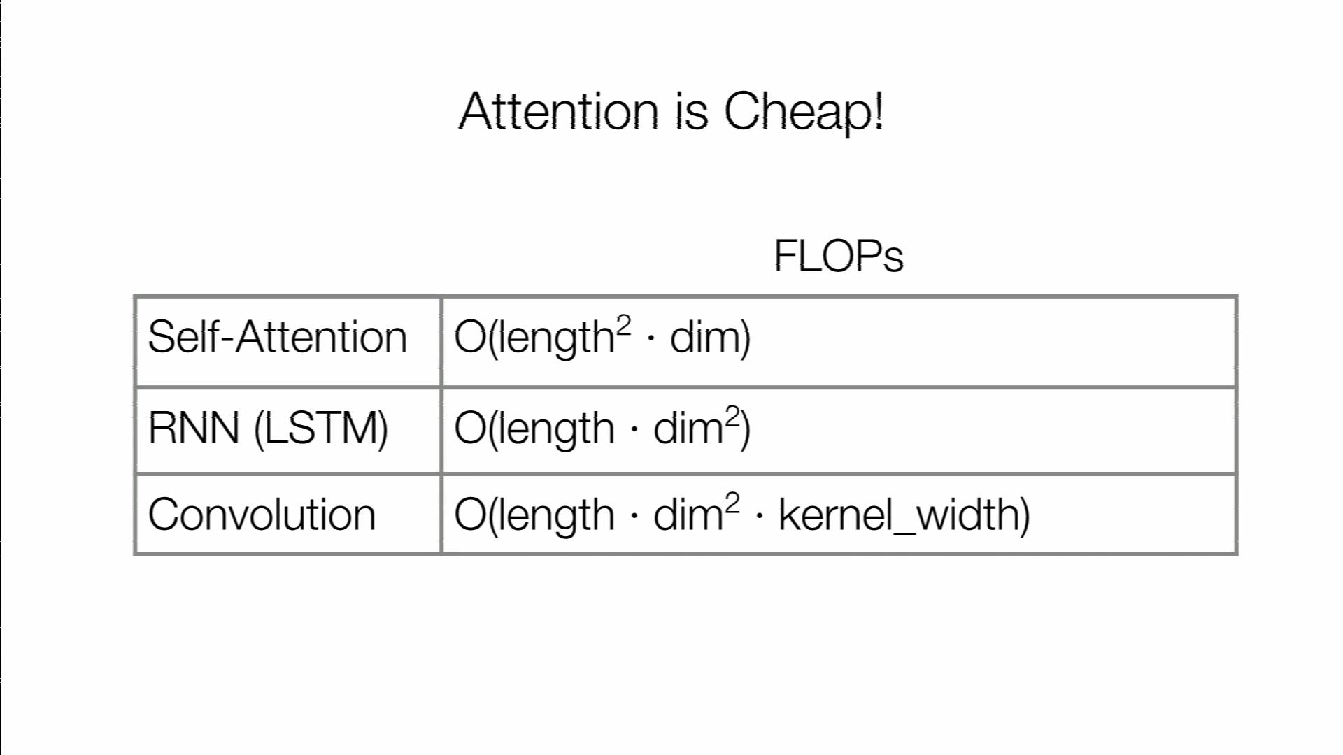
Self-attention is quadratic in sequence length. RNNs and convolutions are quadratic in the model dimension. For sentence-level translation the dimension is larger than the length, so attention is cheaper: he gives roughly four times faster than an RNN, and faster than a width-3 convolution. Most of the rest of the lecture is about what to do when length becomes the larger number.
Multi-head attention: who did what to whom
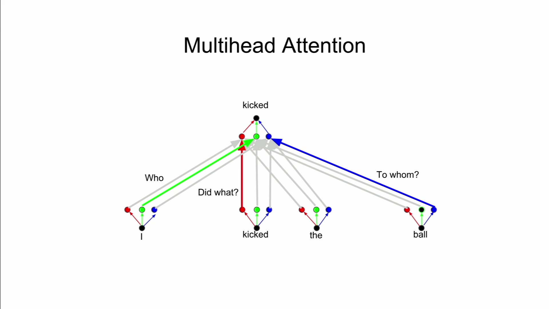
This is the clearest part of the lecture. A convolution applies a different linear transformation at each relative offset, so it can extract different information from “I”, “kicked” and “ball”. A single attention layer applies the same transformation everywhere and can only change the mixing weights. Multiple heads, each with its own projections, act like separate feature detectors: one for who, one for did what, one to whom. To keep the cost flat, each head works in a smaller dimension, so the total FLOPs stay the same and only the number of softmaxes goes up. He suggests that with enough heads, or heads tied to positions, attention could exactly simulate a convolution, at the price of many more parameters.
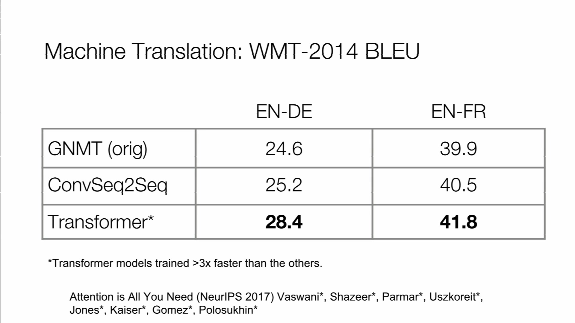
The translation results: 28.4 BLEU on English-German and 41.8 on English-French, ahead of earlier ensembles and trained more than three times faster. He’s careful about what this shows. LSTMs are already universal approximators, so the Transformer isn’t more expressive. “Perhaps all we did was just build an architecture that was good for SGD”, because the gradient path through a weighted sum is simple.
Residuals carry position
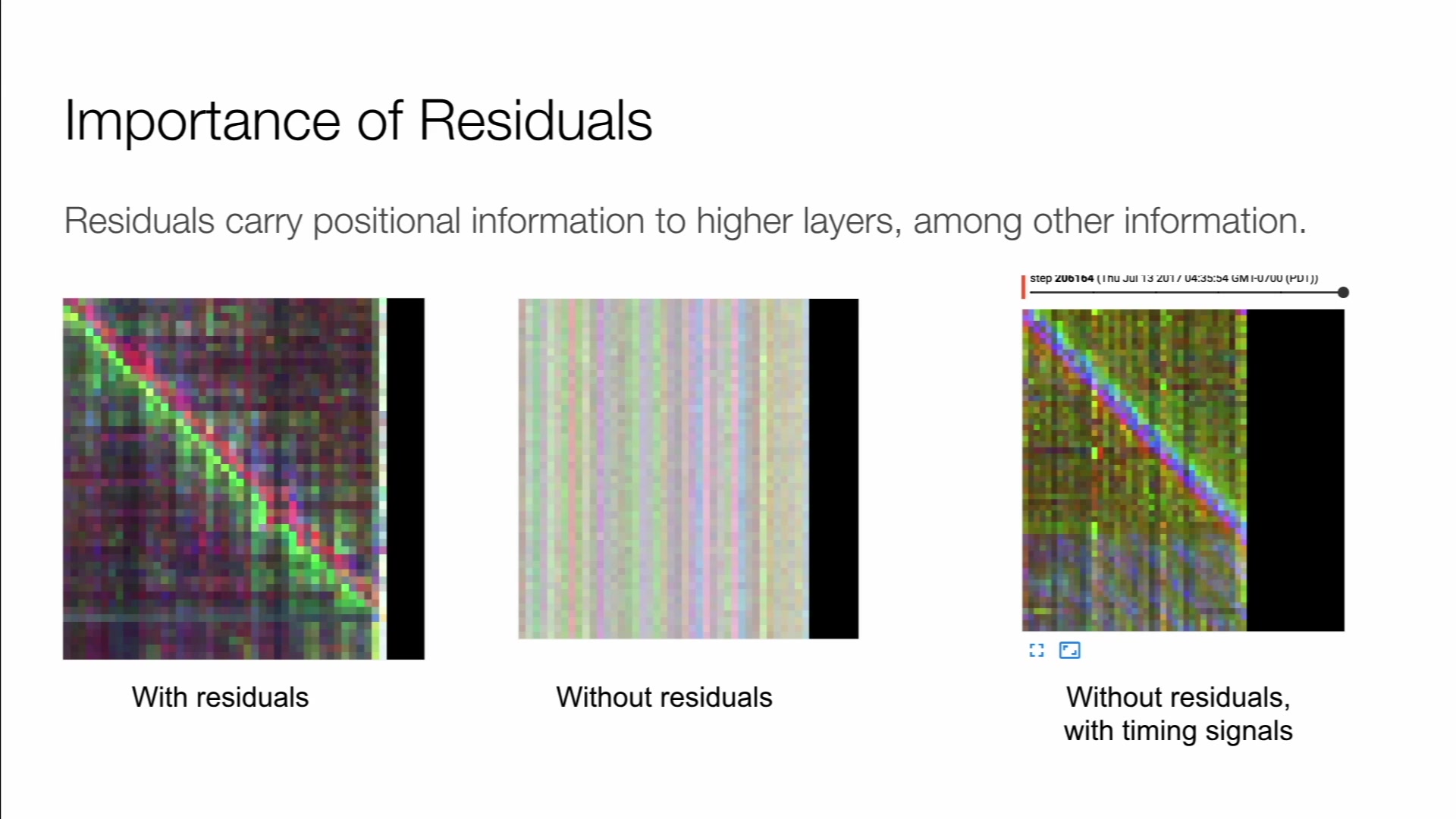
This is a small ablation that’s easy to miss. Position information enters only at the input. When they removed the residual connections, the encoder-decoder attention lost its diagonal shape, because later layers no longer knew where anything was. Adding positional signals back at every layer recovered some of the diagonal but not the accuracy. The residual connections were carrying position information up through the network, along with whatever else they carry.
Images: self-similarity and local windows
The second inductive bias he argues for is self-similarity. Textures repeat at different scales in a Van Gogh, and motifs come back in music. He points out that classic vision techniques already used this: Efros and Leung’s texture synthesis, and non-local means denoising, which rebuilds a patch from similar patches anywhere in the image. Self-attention over pixels is a differentiable version of non-local means.
The Image Transformer treats autoregressive image generation as language modelling over pixels, with 2D position representations. A flattened 32×32×3 CIFAR image is 3,072 positions, so length is now much larger than dimension. The fix borrows from convolutions: restrict attention to local query blocks and memory blocks, in 1D raster order or in 2D tiles. The results were state of the art in likelihood on ImageNet, and on CelebA super-resolution human raters were fooled about four times as often as by earlier work. He’s open that GAN samples looked far better (“the latest GAN result from Nvidia makes us look like a joke”) and argues that the inductive bias is the point.
Music Transformer and relative attention
Anna Huang treats a MIDI performance as a sequence of events: note on, note off, velocity, and clock advances. The comparison is memorable. Given a few bars of a Chopin étude, an LSTM drifts away from the motif almost at once. A vanilla Transformer holds the motif, then falls apart once it passes the length it was trained on. The Music Transformer with relative attention keeps repeating and varying the motif well past that point.
Relative attention (Shaw et al., 2018) adds a term to the attention logits that depends on the distance between query and key, so a head can learn “care about things two beats back” or “care about things a bar ago”, which gives it some translation invariance. Her explanation for the length generalization is that relational information carries forward when absolute positions run out.
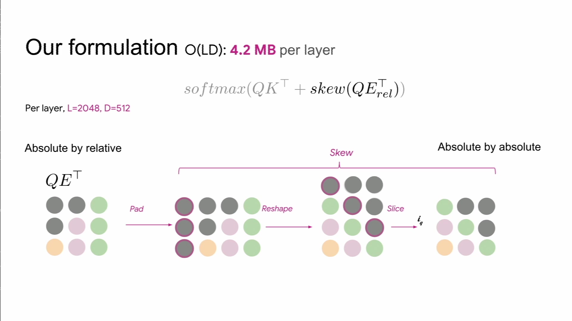
The engineering contribution was memory. Shaw et al. built an L×L×D tensor of relative embeddings, about 8.5 GB per layer at L = 2,048 and D = 512, which is unusable for 2,000-event piano pieces. Huang’s group multiplies queries by the relative embeddings directly, which gives logits indexed by relative distance, and then a pad-reshape-slice “skew” rearranges them into absolute-by-absolute order. The memory cost drops to 4.2 MB per layer.
What Vaswani thought came next
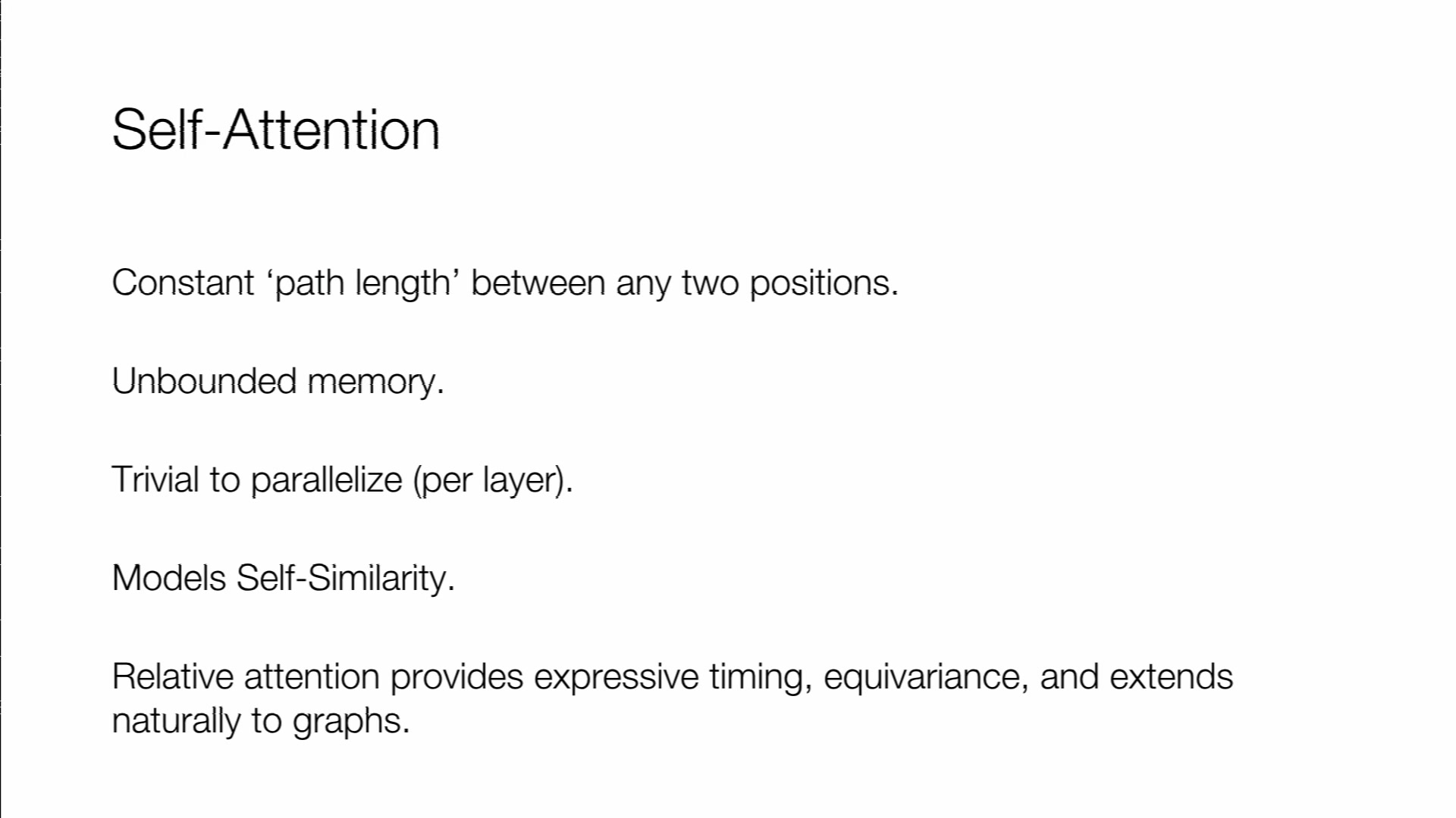
Vaswani closes with connections and open problems. With relative positions and no absolute ones, attention over images becomes translation-equivariant, the property that made convolutions work. Self-attention is message passing on a complete graph, and the “multiple towers” in message-passing neural networks are close to multi-head attention. His open problems are generation that is less autoregressive (non-autoregressive Transformers, iterative refinement, blockwise parallel decoding), larger models via Adafactor and Mesh-TensorFlow, recurrence in depth (Universal Transformers) and across segments (Transformer-XL), self-supervision and transfer, and “surmounting this quadratic problem with self-attention”. Seven years later, most of those are still active research areas.
Key takeaways
- Vaswani’s case for self-attention rests on inductive biases (a constant path length between any two positions, multiplicative gating, and the ability to model self-similarity) as much as on speed.
- Scaled dot-product attention is two matrix multiplications and a softmax. It’s cheaper than RNNs and convolutions whenever sequence length is smaller than model dimension, and much of the field’s later work deals with the opposite case.
- Multiple attention heads let attention extract different information from different positions, as a convolution’s per-offset weights do, without increasing total FLOPs.
- By his own account the Transformer’s win was partly that it is easy for SGD to train, not that it is more expressive than an LSTM.
- Residual connections carry positional information to higher layers. Removing them broke the attention patterns even when position signals were added back at every layer.
- Relative attention let the Music Transformer stay coherent beyond its training length, and the skewing trick cut its memory from O(L²D) to O(LD), from 8.5 GB to 4.2 MB per layer.
- Self-attention can be read as message passing on a fully connected graph, which links Transformers to graph neural networks.
Source
- Lecture: Stanford CS224N, Natural Language Processing with Deep Learning, Winter 2019, Lecture 14: “Transformers and Self-Attention for Generative Models”
- Speakers: Ashish Vaswani (Google Brain), Cheng-Zhi Anna Huang (Google Magenta)
- Recorded: 2019; published by Stanford Online
- Duration: 53:48
- Video: https://www.youtube.com/watch?v=5vcj8kSwBCY