Let's Build GPT From Scratch: Karpathy's Classic, Re-read in 2026

Weekly Video Notes — a short article distilling one talk from the weekly digest. Source video and key frames are embedded throughout.

📜 Classic of the Week. This week’s digest re-surfaces a 2023 classic: Andrej Karpathy’s “Let’s build GPT: from scratch, in code, spelled out.” Three years later it is still, hands down, the clearest single resource for understanding what is actually happening inside a transformer. If you have never sat with it end-to-end, this is your nudge.

Why this video still matters in 2026

Most “explain the transformer” content today either waves at the architecture diagram or buries you in framework abstractions. Karpathy does the opposite: he opens an empty Jupyter notebook, pastes in the tiny Shakespeare corpus, and types out — line by line, ~200 lines total — the same architecture that, scaled up, gave us ChatGPT.

By the end of the 1h56m, you have built nanoGPT: a decoder-only transformer language model that produces vaguely Shakespearean text. More importantly, you understand every tensor shape on the way there. In 2026, with agent frameworks stacked five layers deep on top of LLM APIs, this kind of ground-truth mental model is more valuable, not less.

The talk is also a masterclass in pedagogical sequencing. Each new mechanism is motivated by a concrete shortcoming of the previous one. Let’s retrace the path.

1. Scope and the dataset

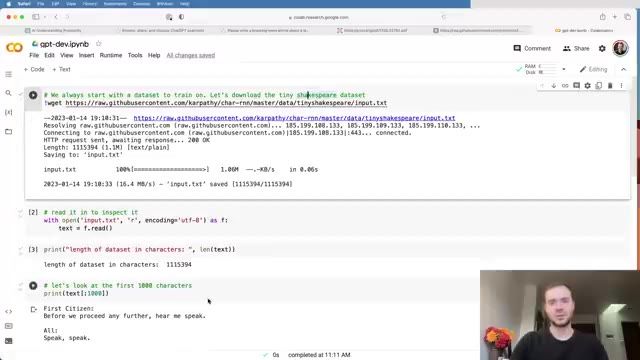
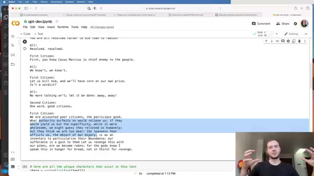
The goal is set explicitly: a character-level language model trained on tiny-shakespeare, a ~1 MB single text file. Character level keeps the vocabulary small (65 unique characters) so you can see every tensor without choking on embedding tables.

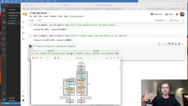
The model is decoder-only (GPT-style), not the full encoder-decoder transformer from Attention Is All You Need. Karpathy is careful about this distinction and returns to it later when explaining what’s missing if you wanted to build a translation model instead.

2. Tokenization and data loading

Tokenization is a one-liner here: build a stoi/itos dict over the 65 characters and define encode/decode as list comprehensions. Karpathy uses this as the opportunity to explain the tradeoff that real systems make — Google’s SentencePiece and OpenAI’s tiktoken use subword BPE, giving shorter sequences for a larger vocabulary. Character-level is the extreme of long sequences over a tiny vocab; production systems sit somewhere in the middle.

The data loader is equally minimal:

• Encode the entire corpus into a torch.LongTensor.
• 90/10 train/val split.
• get_batch samples batch_size random offsets and slices block_size characters as x and the next block_size as y.

block_size (also called context length) and batch_size are the two knobs that govern the shape of everything downstream. He starts with block_size=8, batch_size=4 — small enough to print and stare at.

A subtle but important framing: within a single (x, y) example of length 8, the model is being trained on 8 different prediction problems simultaneously — predict char 1 given char 0, predict char 2 given chars 0..1, and so on. This is what makes the attention masking later both necessary and natural.

3. The bigram baseline

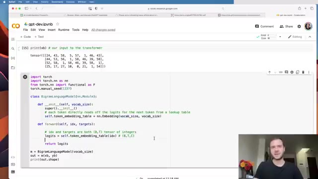
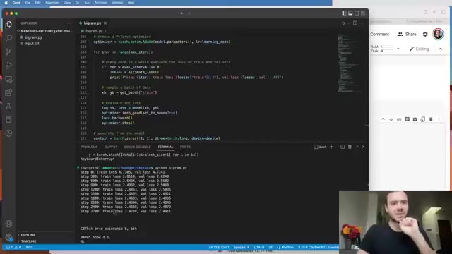
Before any transformer machinery, Karpathy builds a bigram language model as a baseline. It’s just one tensor: a (vocab_size, vocab_size) embedding table where row i directly stores the logits for “what comes after character i”. No context beyond the previous character.

He writes the full training loop here — AdamW, loss.backward(), optimizer.step() — so it’s reusable for everything that follows. The loss drops from -ln(1/65) ≈ 4.17 toward ~2.4. The generated text is gibberish but not random gibberish; you can see character-pair statistics emerging.

This baseline matters because every later mechanism is justified by “the bigram can’t do this, so we need…”.

4. The mathematical trick at the heart of self-attention

Before showing self-attention, Karpathy spends ~20 minutes on what he calls “the mathematical trick” — and it’s the section worth rewinding twice.

The setup: you have a tensor x of shape (B, T, C) — batch, time, channels. For every position t, you want a representation that summarizes positions 0..t (causal, no peeking at the future). The simplest summary is the average of all previous tokens’ embeddings.

The naïve way is two nested for-loops over batch and time. Karpathy then shows three increasingly elegant vectorizations:

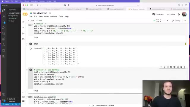
1. Version 2: A lower-triangular matrix of ones, row-normalized, multiplied by x. Matrix multiplication does the averaging in one call.
2. Version 3: Same idea, but build the weights from a zero matrix with -inf above the diagonal, then softmax. The softmax of -inf is 0, of equal values is uniform — so you recover the same averaging.
3. Version 4: Replace the zeros with data-dependent affinities computed from x itself. Now the weights are no longer uniform — they say “how much does position t want to attend to position s?” That is self-attention.

The reason this section is so good is that softmax of -inf for masking is not introduced as a trick to memorize — it falls out as the cleanest way to express “averaging over a prefix” in a way that generalizes to non-uniform weights. By the time you see it as the causal mask in attention, it’s old news.

5. Self-attention, spelled out

With the trick understood, the actual self-attention block is short. Every token at position t emits three vectors via linear projections of its embedding:

• Query — “what am I looking for?”
• Key — “what do I contain?”
• Value — “if you decide I’m relevant, here’s what I’ll contribute.”

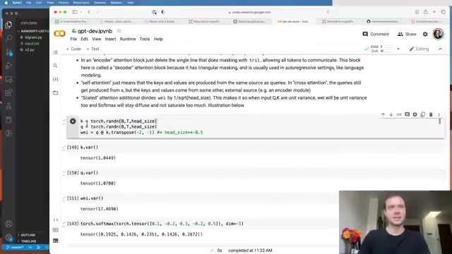
Affinities are dot products of queries with keys, scaled by 1/sqrt(head_size) (the famous scaled in “scaled dot-product attention” — without it, softmax saturates as head_size grows and gradients die). Mask, softmax, multiply by values. That’s it.

Karpathy underlines a few things that are easy to miss:

• Attention has no notion of position. It is a set operation. Position is injected separately via a positional embedding table added to token embeddings.
• Heads are independent communication channels. Multi-head attention is just running several smaller attention operations in parallel and concatenating — it gives the model multiple, specialized “ways of looking” at the past.
• The causal mask is what makes this a decoder. Remove it and you have an encoder block (BERT-style), which can attend bidirectionally — useful for classification, embeddings, encoder-decoder translation, but not autoregressive generation.

6. Multi-head attention + feedforward = the block

A transformer block has two sub-layers:

1. Multi-head self-attention — tokens communicate with each other.
2. Position-wise feedforward — each token independently thinks about what it just heard.

The feedforward is just two linear layers with a ReLU (or GELU) in between, applied independently to every token. Karpathy frames the split as communication vs computation: attention moves information between positions; the MLP transforms it in place.

7. Residual connections and LayerNorm — the things that make it actually train

Stacking blocks naively does not work. Karpathy demonstrates this empirically: deeper models train worse than shallower ones until two tricks are added.

Residual connections. Each sub-layer’s output is added back to its input: x = x + sublayer(x). This creates a “gradient highway” from the loss all the way back to the embeddings, bypassing the (initially poorly behaved) sub-layers. Optimization becomes dramatically easier; loss drops noticeably the moment residuals are added.

LayerNorm. Applied (in modern “pre-norm” style, which Karpathy adopts) to the input of each sub-layer. It normalizes each token’s feature vector to zero mean and unit variance, then applies a learned scale/shift. This keeps activations and gradients well-conditioned across depth.

He also adds dropout as a regularizer once the model is large enough to overfit the tiny dataset — applied inside attention (on the affinities) and on the residual stream.

After these three additions, depth pays off and validation loss keeps dropping.

8. Scaling it up

The final section reuses the exact same code with bigger hyperparameters: batch_size=64, block_size=256, n_embd=384, n_head=6, n_layer=6, dropout 0.2. On a single GPU it trains in about 15 minutes to a val loss around 1.48 and produces text that looks like Shakespeare — wrong words, real cadence, properly formatted speaker tags.

That moment is the punchline of the whole video: the architecture you just built is, modulo scale and data, the same architecture as GPT-3. What changed between this and ChatGPT is not a smarter block — it’s three things:

1. Scale. 10M params → 175B params, and the training corpus from 1 MB of Shakespeare to a substantial fraction of the public internet.
2. Better tokenization (BPE) so the sequence length isn’t strangled by character granularity.
3. A second training stage: this video covers only pre-training (next-token prediction on raw text). That gives you a document completer, not an assistant.

9. What’s next: from document completer to assistant

Karpathy closes by explicitly drawing the line between what was built and what ChatGPT actually is. The post-pretraining stages, which he sketches but does not implement, are:

• Supervised fine-tuning (SFT) — continue training on curated prompt/response pairs so the model learns to answer questions rather than continue text.
• Reward modeling — train a separate model to score responses based on human comparisons.
• RLHF (or now, increasingly, DPO/RLAIF) — use that reward signal to nudge the base model toward preferred behaviors.

He also gestures at encoder vs decoder distinctions, encoder-decoder models (T5, original Transformer for translation), and at the fact that the same backbone, with input/output adapters, underlies most of the multimodal models we now use daily.

Why the talk has aged well

A few things stand out re-watching this in 2026:

• The architecture has barely changed. Most “what’s new” since 2023 — rotary embeddings, grouped-query attention, mixture-of-experts, longer contexts via RoPE scaling, FlashAttention kernels — are optimizations on this same skeleton, not replacements for it. If you know nanoGPT, every modern decoder LLM paper is a small delta.
• The post-training story exploded. What Karpathy sketched in 60 seconds at the end (SFT + RLHF) is now an entire industry, and the open-weights wave (Llama, Qwen, DeepSeek, GLM) has made that stack accessible to anyone.
• Tokenization is still embarrassing. Subword BPE remains the standard and remains the source of most of the dumb-LLM-failure memes (“how many r’s in strawberry”). Karpathy himself later released minbpe as a follow-up; the character-level shortcut in this video deliberately sidesteps the whole problem.
• The “communication vs computation” framing is still the cleanest way to teach what a block does, and it generalizes — graph neural networks, perceivers, and state-space models all separate the two in different proportions.

Key takeaways

1. A GPT is ~200 lines of PyTorch. The architectural budget is tiny; the scale and data are where the magic happens.
2. Self-attention is a weighted average where the weights are learned from the data itself. The causal mask is implemented as softmax(-inf) because that’s the cleanest way to express “average over a prefix” in a differentiable way.
3. Attention has no position; positional embeddings carry that signal. Attention is set-to-set; the time axis is something you add separately.
4. Decoder = causal mask. Encoder = no mask. Same block, different masking, completely different use cases.
5. A block is communication (attention) + computation (MLP). Residuals and LayerNorm are what make it train at depth.
6. Pre-training builds a document completer. Becoming an assistant is a separate, multi-stage process (SFT, RM, RLHF/DPO) that this video doesn’t cover but explicitly names.
7. Mental models compound. In 2026, with agent harnesses, RAG, tools, and observability stacks layered everywhere, knowing what’s actually inside the box pays off every time something behaves weirdly.

Source

📺 Let’s build GPT: from scratch, in code, spelled out. — Andrej Karpathy, January 2023 (~1h56m). Companion repo: karpathy/nanoGPT and the ng-video-lecture notebook.