Weekly Paper Notes — one of the top picks from the 2026-10-31 CS paper digest. Area: AI / ML.
Authors: Randall Balestriero (Brown University, AMI Labs), Yann LeCun (NYU, AMI Labs) arXiv: 2610.39302 · PDF
TL;DR
In 2024 Huh, Cheung, Wang and Isola observed that vision models and language models trained separately end up with increasingly similar representations as they scale, and conjectured that they converge on a shared statistical model of reality. They called it the Platonic Representation Hypothesis (PRH). It was an observation, with no proof and no recipe beyond “scale more”.
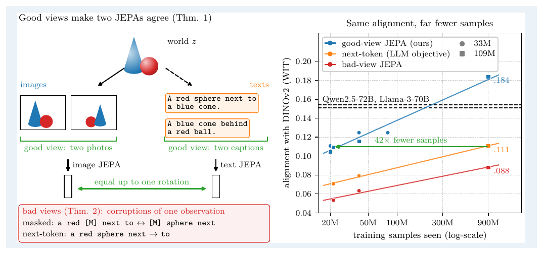
This paper turns it into a theorem for Joint-Embedding Predictive Architectures. If several modalities render the same finite world, and each modality’s JEPA uses positive pairs that relate the same world states, then every one of them learns the same embedding up to a single orthogonal rotation. When the positives differ, the misalignment is bounded by how much their positive-pair graphs differ, divided by a spectral gap.
The useful part is which positives count. Two observations of one scene (two captions of a photo, two frames of a clip) are good views. Two corruptions of one observation (two crops, two maskings of a sentence) are bad views, and they make the encoder spend dimensions on nuisance that no rotation can align. Next-token prediction, the authors show, has the form of a bad-view JEPA: its positives are a prefix and its continuation inside one document.
Empirically, a good-view text JEPA reaches next-token prediction’s alignment with DINOv2 using 42 times fewer samples, and a 109M-parameter BERT-B trained this way scores .184 on the PRH paper’s own benchmark, above every language model they evaluated up to Qwen2.5-72B (.154). One fitted rotation then turns frozen DINOv2 plus a text-only decoder into a captioner reaching CIDEr .838 on COCO.
What problem is the paper actually attacking?
The PRH paper (Huh et al., ICML 2024) measured something real: take a vision encoder and a language model that never saw each other’s data, embed paired images and captions, and the k-nearest-neighbour structure of the two spaces overlaps more as models get bigger. Their explanation was an idealised contrastive learner whose kernel converges to the pointwise mutual information of co-occurring events. That argument fits contrastive learning on bijective observations. It says nothing about the objectives people actually use, and it predicts nothing about when alignment should fail.
There’s an older thread the authors lean on. Word embeddings trained on different languages are related by a linear map (Mikolov et al., 2013), even by a rotation you can find with no parallel data (Conneau et al., 2018). That result always looked like a hint that independently trained encoders were learning the same object in different coordinates.
The other thread is the spectral view of self-supervised learning. HaoChen et al. (2021) showed that spectral contrastive loss learns the top eigenvectors of the “augmentation graph”, the graph whose edges are the positive pairs. Balestriero and LeCun showed in 2022 that VICReg and similar non-contrastive objectives recover spectral embeddings too. If a JEPA with whitening learns the spectral embedding of its positive-pair graph, then the question “do two modalities learn the same thing?” reduces to “do their positive pairs draw the same graph on the world?”
That reduction is the observation the paper is built on. Representations are determined by positives. Scale only enters because, with weak positives, you need a lot of data before the induced graph starts to look like the world’s.
The mechanism: good views versus bad views
The theorem
The setup is deliberately idealised. A world is a finite set of states z with probabilities p(z). Modality m observes it through an injective rendering x = g_m(z), the pixels of a photograph or the tokens of a caption. A JEPA for modality m trains an encoder f on positive pairs (g_m(z), g_m(z')) drawn from a symmetric distribution π_m:
L_m(f) = E_{(z,z')~π_m} ℓ( f(g_m(z)), f(g_m(z')) ) + Ω(f)
The prediction term ℓ and the anti-collapse term Ω are both invariant to rotations. Because the rendering is injective, L_m(f) is just L_π(f ∘ g_m), the same objective written on world states. So if every modality shares the same π and the minimiser is unique up to rotation, every modality’s optimum composed with its renderer equals Q_m h* for one world embedding h* and some Q_m ∈ O(k). That’s Theorem 1, the Platonic Representation Theorem. The proof is two lines once the setup is in place.
Proposition 1 provides the uniqueness. With squared-error prediction and whitening as anti-collapse, the minimisers are exactly Q Φ_π, where Φ_π is the spectral embedding of the normalised adjacency K_π = D^{-1/2} Π D^{-1/2}, provided there’s a gap between the k-th and (k+1)-th eigenvalues. This is Laplacian eigenmaps at the population level. The authors note that LeJEPA’s SIGReg regulariser has the same second moments, but uniqueness under its full-distribution constraint is left as an assumption.
Theorem 2 handles the realistic case where the modalities’ positives differ. The RMS distance between paired embeddings after the best rotation is bounded by:
(2√2 / δ) · min( √k ‖K_π1 − K_π2‖₂ , ‖K_π1 − K_π2‖_F )
with δ the eigengap. On 300 random synthetic worlds the measured error never exceeds 18% of the bound. A corollary that shows up later in the experiments: directions separated by big spectral gaps align, and directions near the tail of the spectrum need not align at all.
Nuisance and why bad views hurt
The injective model can’t express the good/bad distinction because each state has exactly one observation. So the authors add a per-observation nuisance ν (which words a caption happens to use, the camera viewpoint), drawn independently of the state. A good-view JEPA pairs g(z, ν) with g(z', ν') with independent nuisances. A bad-view JEPA pairs two corruptions of one observation, which share the nuisance.
Theorem 3 says that every embedding direction spent on modality-specific nuisance costs alignment: the best-rotation error is at least 2k(1 − min_m ρ(f_m)), where ρ is the fraction of the embedding the world state explains. Proposition 3 says when that happens. A good-view JEPA (under a spectral gap) learns a function of the world state alone, ρ = 1. A bad-view JEPA spends r ≥ 1 directions on nuisance exactly when its corruptions preserve the nuisance more strongly than they preserve the world’s k-th direction. Two crops of one photograph keep its lighting and viewpoint; two spans of one caption keep its wording. Neither of those exists in the other modality.
Theorem 4 then explains the role of data. A bad-view JEPA doesn’t choose its world kernel; the kernel it ends up with depends on which observations happen to overlap after corruption. Weak corruptions mostly pair a caption with itself and only link different captions of the same scene through chains of overlapping fragments, which takes dense data. Strong corruptions link across scenes no matter how much data you have. Good views link every description of a scene in one step and never leave it.
Next-token prediction as a bad-view JEPA
Proposition 4 is the part that will get cited. The next-token loss with a linear softmax head splits as:
−log softmax = −⟨h(c), w_y⟩  +  log Σ_v exp⟨h(c), w_v⟩
               (prediction)     (anti-collapse A(h(c)))
Read this way, it’s a JEPA with a context encoder h, a target encoder y ↦ w_y, inner-product prediction, and positives (c, y) drawn from inside one sequence. The log-partition plays the role of the uniformity term in contrastive learning. At the optimum, h is only identified up to an invertible linear map, not a rotation. The positives are a prefix and its continuation, which share their document’s nuisance (author, wording, style). By the reasoning above, that predicts language models should spend capacity on nuisance and align with vision only slowly, through scale. The authors are careful to call this a heuristic prediction rather than a corollary, since Proposition 3 assumes a single spectral encoder.
Does it hold up? The experiments
The recipe is simple on purpose. Image and text encoders are trained separately with the same LeJEPA objective (invariance to the mean of two global views plus SIGReg, λ = 0.02), and no encoder ever sees the other modality. On Flickr30k the image side is a ViT-S/16 and the text side a 33M-parameter BERT trained three ways that differ only in positives: masked spans of one caption (bad views), spans of different captions of the same image (good views), and causal next-token prediction.
On Flickr test pairs, with one orthogonal map fitted on validation pairs, the good-view text JEPA retrieves the right caption first for 4.4% of images, 44 times chance. Masked spans and next-token prediction land close together and well below it, in every seed. There’s a neat control: next-token prediction trained on concatenated pairs of captions of the same image ([CLS] a [SEP] b [SEP]) barely moves. The same information helps far less as context than as a JEPA view.
The nuisance mechanism can be measured directly, since every Flickr image has five captions. For k = 32 the scene explains .804 of the good-view embedding, .655 of the bad-view JEPA and .608 of next-token prediction. Plugging those into Theorem 3 gives lower bounds on best-rotation error against DINOv2 of 12.6, 22.1 and 25.1; the measured errors are 33.5, 39.4 and 40.3, in the same order.
An ablation finds that trimming does most of the work. Using whole captions as views loses about a quarter of the alignment, while masking rate, number of views, batch size and width move the result by about as much as seed noise. Training needs gradient clipping, though: without it, 3 of 36 runs collapsed abruptly between epochs 20 and 60.
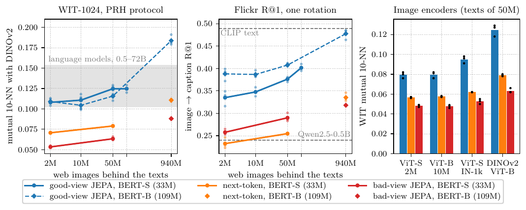 Good views scale on web text. Left: alignment with DINOv2 on the PRH paper’s WIT-1024 benchmark as the text JEPA trains on texts of 2.16M to 940M Recap-DataComp images; the 109M model at 940M (dashed) clears the language-model band. Middle: Flickr retrieval through one rotation, without ever seeing a Flickr caption. Right: the ordering holds across image encoders trained from scratch and frozen DINOv2. Source: Balestriero, LeCun — arXiv:2610.39302, Figure 9.
At scale, the text side trains on Recap-DataComp, where each image contributes its alt-text and two LLaVA recaptions as views. With the same 109M encoder and corpus, the good-view JEPA reaches WIT alignment .109 after 21.6M samples; next-token prediction reaches .111 after 900M. That’s the 42× figure (14× in tokens, since a good-view sample reads three texts). Trained on all 940M images, the good-view BERT-B scores .184 mutual 10-NN with DINOv2 ViT-B, against .154 for Qwen2.5-72B, .151 for Llama-3-70B and .124 for CLIP’s text encoder. It also leads with CLIP ViT-H/14, MAE and I-JEPA as the vision side.
Alignment follows a fitted scaling law in the fraction q of good-view items and the samples seen M, R@1 = a + d log M + b log(1 + q^α M^β N^γ / c). Fitted on 45 cells, it predicted 85 new runs before training them with RMSE .0093, the same as seed-to-seed variation. It breaks further out (overestimating at 320M samples with heavy data repetition), and the authors label it an empirical summary of one recipe, not a consequence of the theory.
What the rotation buys you
If two encoders really agree up to a rotation, you can compose them. The authors train a caption decoder on text alone, reconstructing captions from frozen good-view JEPA embeddings with Gaussian noise added. To caption an image they embed it with frozen DINOv2, apply the rotation, and decode. The noise level isn’t tuned; it’s set from the residual cosine after rotation, σ = (c⁻² − 1)^{1/2} ≈ 3. With a larger decoder (Qwen2.5-1.5B fine-tuned on text), DINOv2 ViT-g plus DINOv3 features and consensus over 32 samples, the system reaches CIDEr .838 on COCO, while the only parameters fitted on image–caption pairs are those of one map with orthonormal rows. Replacing the rotation with an unconstrained linear map fits Flickr slightly better but loses a fifth on COCO, which is the behaviour you’d expect if the spaces really are related by a rotation.
You can also find the rotation with no pairs at all. Running the unchanged code of Schnaus et al. (2026), which matches cluster geometry and refines by optimal transport, the 109M good-view JEPA reaches 64.4% top-5 zero-shot on ImageNet-100, against 47.6% for Qwen3-8B rerun under identical conditions. Next-token prediction on the same texts fails in about half its runs.
Caveats the authors state
The theorems are population statements on a finite world with injective renderings and matched marginals; real modalities are lossy, and a caption sees only part of a photo. Uniqueness up to rotation is proved for whitening, not for LeJEPA’s SIGReg, which the experiments use. The image side is mostly a bad-view JEPA itself (DINOv2’s positives are crops), and the one test with good image views (MSR-VTT frames) uses a weak 7k-clip encoder.
The biggest caveat is where good views come from. On Recap-DataComp two of each image’s three texts are written by LLaVA on LLaMA-3-8B, whose vision tower is CLIP ViT-L/14, so paired image–text information leaks in through the data. Without any captioner (alt-text plus a text-only paraphrase) WIT alignment drops from .107 to .060. The comparisons between objectives on identical texts don’t depend on this; the headline comparison against 72B language models does. Hyperparameters were also tuned only for the good-view JEPA, and one of four 940M seeds, trained with a different SIGReg weight, scored .121.
Why this matters
For a hypothesis that has mostly been discussed as a philosophical curiosity, this is a concrete reframing. Alignment between modalities becomes a property of the positive-pair graph, and you can engineer the graph. That gives practitioners a knob that isn’t “add parameters”, and it gives a principled account of why the PRH paper’s curves looked like scaling curves: language models get their positives from within-document continuations, which only approximate the world’s kernel after enormous amounts of text.
It’s also, unsurprisingly given the authors, an argument against next-token prediction as the route to grounded representations. I’d read the 72B comparison with the recaptioner caveat in mind, but the controlled comparisons on identical text are clean and consistent across Flickr, MSR-VTT and web scale. The obvious follow-ups are good image views at scale (multiple photographs or frames of one scene), audio and action modalities, and whether the same view construction helps when an LLM is the text side rather than a small BERT.
Read alongside
- Huh, Cheung, Wang, Isola, The Platonic Representation Hypothesis (ICML 2024), the conjecture and the WIT-1024 benchmark used here.
- HaoChen, Wei, Gaidon, Ma, Provable Guarantees for Self-Supervised Deep Learning with Spectral Contrastive Loss (NeurIPS 2021), the augmentation-graph view behind Proposition 1.
- Assran et al., Self-Supervised Learning from Images with a Joint-Embedding Predictive Architecture (I-JEPA, CVPR 2023).
- Balestriero, LeCun, Contrastive and Non-Contrastive Self-Supervised Learning Recover Global and Local Spectral Embedding Methods (NeurIPS 2022).
- Balestriero, LeCun, LeJEPA: Provable and Scalable Self-Supervised Learning Without the Heuristics (2025), the SIGReg objective used in every experiment.
- Conneau et al., Word Translation Without Parallel Data (ICLR 2018), the cross-lingual rotation result this generalises.
- Oquab et al., DINOv2: Learning Robust Visual Features without Supervision (2023), the frozen vision side in most comparisons.
Links
📄 arXiv abstract · 📄 PDF
Part of the Weekly CS Paper Digest series. Summary written from a close read of the preprint; figures cropped from the arXiv PDF and reproduced here under fair use for educational commentary.