Weekly Paper Notes — one of the top picks from the 2026-08-22 CS paper digest. Area: AI / ML.
Authors: Nayeon Kim, Hojin Lee, Yunju Bak, Jaesun Park, Boseop Kim, et al. arXiv: 2608.20061 · PDF · Published at COLM 2026
TL;DR
Choosing the learning rate for a frontier pretraining run is one of the highest-stakes, least-principled decisions in the field. At trillion-token scale a single sweep is unaffordable, so labs guess, extrapolate by folklore, or burn compute they’d rather spend on tokens. Maximal Update Parameterization (μP) solved half of this in 2021 by making the optimal learning rate transfer across model width — tune on a small proxy, apply to the large model. But μP says nothing about the token axis, and modern runs are defined as much by their 10T-token horizons as by their parameter counts.
This paper composes the two axes into a single practical recipe. Step one: adapt μP to a Mixture-of-Experts architecture using Multi-head Latent Attention and the Muon optimizer — a combination that is not covered by existing μP results — and verify that the optimal learning rate transfers across 2×, 4×, and 8× width scalings. Step two: establish a learning-rate scaling law along the token dimension by fitting second-order polynomials of validation loss versus $\log \eta$ at many token budgets, taking each parabola’s vertex as the optimal rate, then regressing those optima against token budget in log-log space.
The fit achieves $R^2 = 0.95$ and extrapolates to an optimal learning rate of $3.85 \times 10^{-4}$ for a 10-trillion-token horizon. The authors then actually spent the compute: they pretrained a 155B-total / 17B-active MoE foundation model from scratch on 10T tokens using that predicted rate. Full-scale pretraining required roughly 98× the total compute of the proxy runs that produced the prediction. The loss curve is smooth, and the resulting model is competitive with DeepSeek-V4-Flash, Hunyuan-A13B, and dots.llm1 on MMLU-Pro.
What problem is the paper actually attacking?
The lineage here is clean and worth stating precisely, because the paper’s contribution is exactly the gap between two well-known results.
μP and μTransfer (Yang & Hu, 2021; Yang et al., 2022) established that under a specific parameterization — width-dependent initialization variances and per-parameter-group learning rate scaling factors — the optimal learning rate becomes invariant to model width. Tune a 40M-parameter proxy, transfer to 6.7B. This was a genuine breakthrough and is now standard practice at labs that can implement it correctly.
But μP has two boundaries the frontier has since crossed. First, the published transfer results are for dense transformers with standard attention and Adam-family optimizers. Modern frontier models are sparse MoE, increasingly use Multi-head Latent Attention to compress the KV cache, and are increasingly trained with Muon rather than AdamW. The paper notes that μP has been extended to Muon in prior work (Shah et al., 2025), but the specific composition — MoE sparsity scaling + MLA’s fixed low-rank projections + Muon — is unaddressed, and each of those pieces perturbs the fan-in/fan-out bookkeeping that μP depends on.
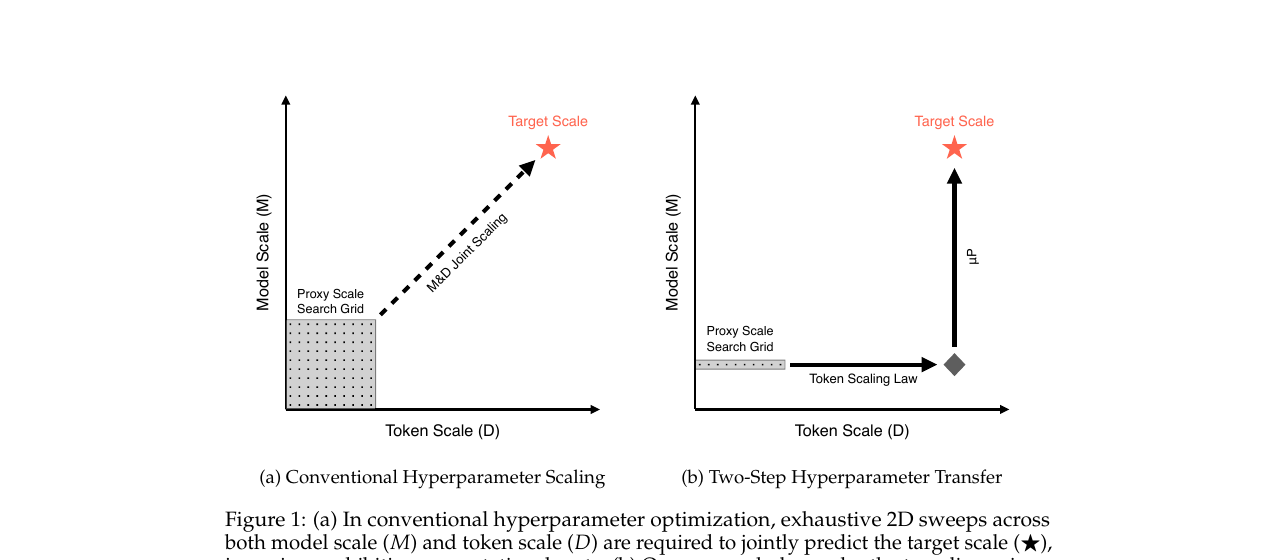
Second, and more fundamentally, μP transfers across width, not across token budget. The optimal learning rate for a 500B-token run is not the optimal learning rate for a 10T-token run, and no amount of width transfer tells you the difference. Since you cannot afford a sweep at 10T tokens even with a tiny model, this axis has been handled by intuition.
The observation that motivates the whole framework: if the two axes can be decoupled — width handled by μP, tokens handled by a fitted scaling law — then a single cheap set of proxy runs suffices to determine both, and the search collapses from a 2D grid to two independent 1D problems.
The mechanism: μP for MLA-MoE, then a token-axis scaling law
Step 1 — μP adapted to MoE with MLA
μP works by classifying every parameter tensor by its shape invariance to width and applying the corresponding initialization and learning-rate scaling. The paper’s classification:
- Vector-like — parameters with exactly one infinitely expandable dimension: embeddings, all biases, and — notably — expert FC2 weights.
- Matrix-like — parameters with two infinitely expandable dimensions: FFN, attention, router, and expert FC1 weights.
The expert FC2 classification is the non-obvious call. Those weights are treated as vector-like because their effective input dimensionality remains bounded by the fixed number of active experts and the fixed MoE intermediate dimension, even as the model widens. The scaling rules follow:
| I/O Embeddings & All Biases (vector-like) | Hidden Weights (vector-like) | Hidden Weights (matrix-like) | |
|---|---|---|---|
| Init. variance | 0.04 | $\text{fan_in}_{\text{base}}/\text{fan_in}$ | $\text{fan_in}_{\text{base}}/\text{fan_in}$ |
| LR scaling factor | 1 | 1 | $\text{fan_in}_{\text{base}}/\text{fan_in}$ |
There’s a neat degenerate case for MLA. The low-rank projection dimensions for query and key-value are held fixed during width scaling. Since those dimensions serve as the fan-in of the corresponding up-projection matrices, the learning-rate scaling applied to those matrices reduces to 1 and has no effect. MLA’s architecture partly sidesteps the question.
The MoE scaling path matters too. When scaling up, the authors fix the number of active experts per token and the MoE intermediate dimension, while increasing the total expert count and hidden dimension. This mirrors how MoE models are actually scaled in practice — raising sparsity to increase capacity while keeping per-token inference cost flat. Total scale, active scale, and sparsity therefore become coupled rather than independent axes. The authors argue this remains μP-compatible via the spectral-condition view: changing the active ratio by adding experts introduces no change to any individual expert’s fan-in or fan-out beyond that already induced by width scaling.
There’s a pleasing practical consequence. Very high sparsity is hardware-inefficient at proxy scale due to low arithmetic intensity, so you want to run the proxy search at lower sparsity and transfer to a higher-sparsity target — which this scaling rule permits.
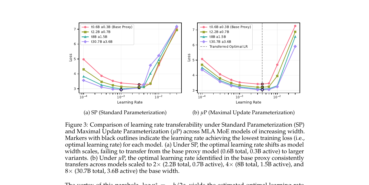
The empirical check is Figure 3, and it is unambiguous:

Under SP, the optimum shifts as width grows from the 0.6B-total/0.3B-active base proxy through 2.2B/0.7B, 8B/1.5B, and 30.7B/3.6B. Under μP, it doesn’t move.
Step 2 — the token-axis scaling law
Here the paper does something more delicate than it first appears. To estimate the optimal rate at a given token budget you need a clean loss signal, but raw checkpoints are noisy. The authors apply an exponential moving average over weights:
$$\theta_{\text{EMA}}^{(t)} = \alpha \cdot \theta_{\text{EMA}}^{(t-1)} + (1-\alpha) \cdot \theta^{(t)}$$
with $\alpha = 0.6$, updated at ~2B-token intervals, analyzing every 10B tokens. Under the effective-decay-window definition of Baidu-ERNIE-Team (2025), this means the most recent 20B tokens retain more than 1% influence on the merged weights.
For each token scale $B$, validation loss on a fixed batch is modelled as a second-order polynomial in the log learning rate:
$$L(\eta) = a(\log \eta)^2 + b(\log \eta) + c$$
The vertex $\log \eta^* = -b/2a$ gives the estimated optimum $\eta^* = \exp(-b/2a)$ for that budget. Then the token-axis law is a straight line in log-log space:
$$\log(\eta^*) = \beta \cdot \log(B) + \gamma$$
Two methodological choices deserve credit. First, the WSD (Warmup-Stable-Decay) scheduler is used to match the target long-horizon setup, and the EMA merge substitutes for the prohibitively expensive alternative of running a separate decay phase per proxy point. Second, when batch-size scheduling is in play, the regression is restricted to data points collected after training dynamics stabilize following the batch-size increase — avoiding transient artifacts that would corrupt the fit.
The paper is also explicit about what it excludes: batch size. This is argued, not hand-waved. Batch size is not merely a modeling hyperparameter but a system-level variable adjusted to maximize hardware throughput, and the literature genuinely disagrees on how it scales — some work ties optimal batch size to training compute, other work to token budget alone, with parallel contradictions in critical-batch-size estimation. Rather than build on contested ground, the authors fix batch size for GPU efficiency and derive a learning-rate law that holds regardless of that choice.
Why the search stays cheap (the practical claim)
The economics are the entire point. The base proxy is a 10.8B-total / 3.3B-active model — one-quarter the width of the 155B-total / 17B-active target — trained for approximately 500B tokens. Optimal rates are estimated at 10B-token intervals using the EMA weights.
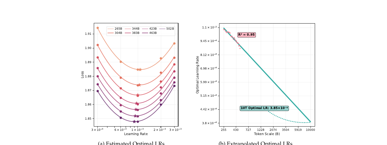
The regression is fitted only to budgets after 255B tokens — again, to ensure post-batch-size-increase stability — and extrapolates across roughly 20× beyond the largest observed budget (502B → 10T). That is an aggressive extrapolation, and the authors know it; they provide additional held-out validation in an appendix.
Against this, full-scale pretraining of the 155B/17B target over 10T tokens costs about 98× the total compute of the proxy runs. The framework’s claim is that this 98× is spent once, on training, rather than partially on search.
Results
The headline validation is not a benchmark table — it’s that they committed. The predicted $3.85 \times 10^{-4}$ was used to pretrain the 155B-total / 17B-active foundation model from scratch over the full 10T-token Stage 1 horizon.
Loss trajectory. The training loss curve descends smoothly from ~1.7 to ~1.3 across the 10T tokens with no instability spikes, no divergence, and no manual intervention reported. For anyone who has watched a frontier run blow up at 3T tokens, this is the result that matters.
Data mixture. Stage 1 begins at 45% English, 27.5% Code, 12.5% Math/STEM, 15% Multilingual. At the 6T-token mark the mixture shifts to 22.5% English, 27.5% Math/STEM, 25% Code, 25% Multilingual to strengthen underrepresented domains. Worth noting that this mid-run mixture change did not destabilize training under the predicted rate.
Downstream benchmarks. After Stage 1, the model is evaluated across four domains: English (MMLU, MMLU-Pro, BBH), Multilingual (Global-MMLU in Korean, Japanese, Vietnamese, Chinese), Math (MATH, GSM8K), and Code (MBPP, HumanEval). On MMLU-Pro the model sits in the same competitive band as DeepSeek-V4-Flash, Hunyuan-A13B, and dots.llm1 — the relevant comparison set for MoE models in this active-parameter class.
The honest caveat, stated by the authors. Running an exhaustive full-scale sweep to definitively verify that $3.85 \times 10^{-4}$ was optimal is computationally infeasible. What they offer instead is the exceptionally stable loss trajectory and competitive downstream performance as strong circumstantial evidence. This is the right way to report it — the counterfactual genuinely cannot be purchased.
Why this matters
Scaling laws have mostly been descriptive: given compute, here’s the loss you should expect. This paper is part of a shift toward prescriptive scaling laws — given your target, here’s the hyperparameter to use — and prescriptive laws are worth more, because they change what you do rather than what you predict.
The specific unlock is that the search cost for a frontier pretraining run becomes roughly independent of the run’s scale. You pay for proxy models at 1/4 width and 1/20 the token horizon, fit two curves, and go. For organizations that are not OpenAI or Google, that difference determines whether a from-scratch frontier MoE run is attemptable at all. The paper is transparently a methods-plus-artifact writeup from a lab that used this to ship a model, which is the most credible form such a paper can take.
The composition insight generalizes beyond learning rate. The pattern — identify a hyperparameter whose optimum is invariant along one axis via principled parameterization, then fit an empirical law along the orthogonal axis — is a template. Batch size is the obvious next target, and the authors’ own framing of why they excluded it reads like a research agenda: settle whether optimal batch size depends on compute or token budget, and the same two-step structure applies.
The limitations the authors name are the right ones. The framework is validated for MLA-based MoE with Muon; extending it to other architectures and optimizers is future work, and given how much of the μP bookkeeping depends on architectural specifics, that extension is not free. And the 20× token extrapolation, while well-supported, is the load-bearing assumption. A follow-up that tests the law’s fidelity at intermediate scales — say, predicting 2T from 500B and then actually training at 2T — would convert the strongest circumstantial evidence into direct evidence.
Read alongside
- “Tensor Programs V: Tuning Large Neural Networks via Zero-Shot Hyperparameter Transfer” (Yang et al., 2022) — the μTransfer paper this work extends; essential for understanding the parameter classification table.
- “Feature Learning in Infinite-Width Neural Networks” (Yang & Hu, 2021) — the theoretical foundation of μP.
- “Muon: An Optimizer for Hidden Layers in Neural Networks” (Jordan et al., 2024) — the optimizer used throughout, and part of why existing μP results didn’t directly apply.
- DeepSeek-V2 / MLA (Liu et al., 2024) — the origin of Multi-head Latent Attention, whose fixed low-rank projections interact with μP scaling in the way described above.
- “MiniCPM” / WSD scheduler (Hu et al., 2024) — the Warmup-Stable-Decay schedule whose extended stable phase makes the EMA-merge estimation trick viable.
- “Scaling Laws for Neural Language Models” (Kaplan et al., 2020) and Chinchilla (Hoffmann et al., 2022) — the descriptive scaling-law tradition this paper turns prescriptive.
Links
📄 arXiv abstract · 📄 PDF
Part of the Weekly CS Paper Digest series. Summary written from a close read of the preprint; figures cropped from the arXiv PDF and reproduced here under fair use for educational commentary.